A tool to assess water resources availability in a river basin.
Water is vital for sustaining food security, industry, power generation, etc. in river basins. But terrestrial and aquatic ecosystems are also very dependent on water to provide valuable ecosystem services, today and tomorrow. Being able to manage the complex flow paths of water to and from all these different water use sectors, as well as their consumptive use, requires a quantitative understanding of the hydrological processes.
Innovative information systems are thus necessary to help managers to manage water consumption more tightly – following certain well defined targets – and to understand which flows to manipulate by means of retention, withdrawals and land-use change. Managers need background data to help them to optimise water allocation to sectors without further depleting the natural capital in a basin. The Google Earth Engine provides operational products that can be used to assess water resources in a river basin.
Step 1: copy the template into a new script and fill in the author details, date and contact information.
Step 2: import the Chirps image collection.
Step 3: Setup the period of interest.
// variables for start and end year
var startyear = 2000;
var endyear = 2016;

// variables for start and end month
var startmonth = 1;
var endmonth = 1;

// define start and end date
var startdate = ee.Date.fromYMD(startyear,startmonth,1);
var enddate = ee.Date.fromYMD(endyear+1,endmonth,1);

// create list for years
var years = ee.List.sequence(startyear,endyear);
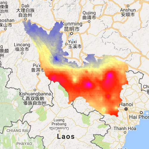
Step 4: Upload the polygon map of the Red river as a fusion table and import it into the GEE.
// polygon for the red river
var redriver = ee.FeatureCollection()
Step 5: Select the data for the period of interest
// select precipitation for time range
var P = chirps.filterDate(startdate, enddate)
  // Sort chronologically in descending order.
  .sort('system:time_start', false)
  .filterBounds(redriver);
Step 6: Include the snippet below to calculate the yearly amount of precipitation. What do we need at the location of the ???? Min, max, mean, sum?
// calculate yearly P
var yearlyP =  ee.ImageCollection.fromImages(
  years.map(function (y) {
  var w = P.filter(ee.Filter.calendarRange(y, y, 'year')).???();
  return w.set('year', y)
                        .set('date', ee.Date.fromYMD(y,1,1))
                        .set('system:time_start',ee.Date.fromYMD(y,1,1));

}));
Step 7: Now we are going to setup the visualization for an image and a barchart.
// set visualizaton parameters
var p_viz = {min:0.0, max:2400, palette:"000000,0000FF,FDFF92,FF2700,FF00E7"};

// Predefine the chart titles.
var title = {
  title: 'Yearly precipitation',
  hAxis: {title: 'Time'},
  vAxis: {title: 'Precipitation (mm)'},
};
Step 8: We create a chart from the yearly precipitation data, using the redriver polygon as the area and a reducer to calculate the mean precipitation in that area.
var chart = ui.Chart.image.seriesByRegion(yearlyP, redriver, ee.Reducer.mean(), 'precipitation', 2500, 'system:time_start', 'SITE')
    .setOptions(title)
    .setChartType('ColumnChart');
Step 9: Display the result. What do we need at the location of the ???? Min, max, mean, sum?
// plot the chart
print(chart)

// center the map
Map.centerObject(redriver, 5);

// plot the map
Map.addLayer(yearlyP.????.clip(redriver),p_viz, "mean yearly P")
We are going to calculate the average monthly precipitation. This needs to be done in two steps:
1. calculate the total precipitation for each month using sum()
2. Calculate the average monthly precipitation using mean().
Step 10: Use the snippet below to calculate the total monthly precipitation. Adjust the graph to display the monthly P. Also adjust the map display.
// Make a list with months
var months = ee.List.sequence(1,12);

// calculate the total amount of precip for each month
var allP =  ee.ImageCollection.fromImages(
  years.map(function (y) {
  return months.map(function(m){
  var w = P.filter(ee.Filter.calendarRange(y, y, 'year'))
           .filter(ee.Filter.calendarRange(m, m, 'month'))
           .sum();
  return w.set('year', y)
           .set('month', m)
           .set('date', ee.Date.fromYMD(y,m,1))
           .set('system:time_start',ee.Date.fromYMD(y,m,1))

});
}).flatten());
Step 11: Calculate the mean monthly precipitation. Adjust the graph and display again.
// calculate monthly P
var monthlyP =  ee.ImageCollection.fromImages(
  months.map(function (m) {
  var w = allP.filterMetadata('month', 'equals', m).mean();
  return w.set('month', m)
          .set('date', ee.Date.fromYMD(1,m,1))
          .set('system:time_start',ee.Date.fromYMD(1,m,1));
}).flatten());
Actual evapotranspiration is the amount of water evaporated from the surface or transpired by plants. As this represents a large portion of the total water balance, it is important to include it.
Step 11: Create a new script.
Step 12: Import the evapotranspiration data.
// import ET data
var ET = ee.ImageCollection("users/atepoortinga/etdata")
Step 13: Display the ET data.
print(ET)

var et_viz = {min:0.0, max:150, palette:"000000,0000FF,FDFF92,FF2700,FF00E7"};
Map.addLayer(ee.Image(ET.mean()), et_viz, "Mean ET");
1. What are the areas with high and a low ET?
2. What is the period covered by ET data?
Step 14: Use the previous script to display a chart with the monthly averages.
1. What are the months with the highest and lowest evapotranspiration?
Tip! You can open several tabs with the google earth engine to easy copy and paste code.
Now we are going to calculate the effective rainfall. Effective rain is the amount of rain that is not evaporated.
Step 15: Create a new script and import the ET and chirps data.
Step 16: Combine both datasets into a new image collection and calculate the effective rainfall.
// calculate the et for each month
var allET =  ee.ImageCollection.fromImages(
  years.map(function (y) {
  return months.map(function(m){
  var w = ET.filter(ee.Filter.calendarRange(y, y, 'year'))
           .filter(ee.Filter.calendarRange(m, m, 'month'))
           .sum();
  return w.set('year', y)
           .set('month', m)
           .set('date', ee.Date.fromYMD(y,m,1))
           .set('system:time_start',ee.Date.fromYMD(y,m,1))

});
}).flatten());

// calculate the P for each month
var allP =  ee.ImageCollection.fromImages(
  years.map(function (y) {
  return months.map(function(m){
  var w = P.filter(ee.Filter.calendarRange(y, y, 'year'))
           .filter(ee.Filter.calendarRange(m, m, 'month'))
           .sum();
  return w.set('year', y)
           .set('month', m)
           .set('date', ee.Date.fromYMD(y,m,1))
           .set('system:time_start',ee.Date.fromYMD(y,m,1))

});
}).flatten());
// combine the two datasets
var myCollection = allP.combine(allET);

print(myCollection)

// calculate the effective rainfall
myCollection = myCollection.map(function(img){
  var myimg = img.expression("(p - et) ",
  {
    p: img.select("precipitation"),
    et: img.select("b1"),
    });
  return img.addBands(myimg.rename('effective_rainfall'));
})

// setup the chart
var chart = ui.Chart.image.seriesByRegion(myCollection, redriver, ee.Reducer.mean(), 'effective_rainfall', 2500, 'system:time_start', 'SITE')
    .setOptions(title)
    .setChartType('ColumnChart');
Step 16: Create an image and chart of the results.
Assignment 1: Compare the monthly effective rainfall with the discharge measured in Son Tay. Do also a comparison on the yearly timescale. Use 165,201 km2 as total area of the basin
Assignment 2: Do a similar type of analysis for your particular basin of interest.
See an example here
