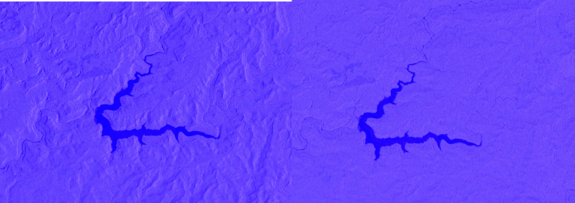
Step 1: Applying terrain corrections to Sentinel-1
Radiometric distortions over rugged terrain within the backscatter products on GEE originate from the side-looking SAR imaging geometry and are strong enough to exceed weaker differences of the signal due to variation in land cover —

Vollreath, Mulissa and Reiche did some great work to account for the radiometric terrain distortions in the earth engine. We use their work as a first pre-processing for surface water mapping. Find the code below or follow the link.
// Import Sentinel-1 Collection
var s1 =  ee.ImageCollection('COPERNICUS/S1_GRD')
			.filter(ee.Filter.listContains('transmitterReceiverPolarisation', 'VH'))
			.filter(ee.Filter.listContains('transmitterReceiverPolarisation', 'VV'))
			.filter(ee.Filter.eq('orbitProperties_pass', 'DESCENDING'))
			.filter(ee.Filter.eq('instrumentMode', 'IW'))
			.filterBounds(geometry)
			.filterDate("2020-10-01","2020-10-31");

var firstNoTerrainCorrection = ee.Image(s1.first());

Map.addLayer(firstNoTerrainCorrection,{min:-25,max:20},"no terrain correction");

s1 = s1.map(terrainCorrection);

var firstTerrainCorrection = ee.Image(s1.first());

Map.addLayer(firstTerrainCorrection,{min:-25,max:20},"Terrain corrected");


// Implementation by Andreas Vollrath (ESA), inspired by Johannes Reiche (Wageningen)
function terrainCorrection(image) {
  var imgGeom = image.geometry()
  var srtm = ee.Image('USGS/SRTMGL1_003').clip(imgGeom) // 30m srtm
  var sigma0Pow = ee.Image.constant(10).pow(image.divide(10.0))

  // Article ( numbers relate to chapters)
  // 2.1.1 Radar geometry
  var theta_i = image.select('angle')
  var phi_i = ee.Terrain.aspect(theta_i)
    .reduceRegion(ee.Reducer.mean(), theta_i.get('system:footprint'), 1000)
    .get('aspect')

  // 2.1.2 Terrain geometry
  var alpha_s = ee.Terrain.slope(srtm).select('slope')
  var phi_s = ee.Terrain.aspect(srtm).select('aspect')

  // 2.1.3 Model geometry
  // reduce to 3 angle
  var phi_r = ee.Image.constant(phi_i).subtract(phi_s)

  // convert all to radians
  var phi_rRad = phi_r.multiply(Math.PI / 180)
  var alpha_sRad = alpha_s.multiply(Math.PI / 180)
  var theta_iRad = theta_i.multiply(Math.PI / 180)
  var ninetyRad = ee.Image.constant(90).multiply(Math.PI / 180)

  // slope steepness in range (eq. 2)
  var alpha_r = (alpha_sRad.tan().multiply(phi_rRad.cos())).atan()

  // slope steepness in azimuth (eq 3)
  var alpha_az = (alpha_sRad.tan().multiply(phi_rRad.sin())).atan()

  // local incidence angle (eq. 4)
  var theta_lia = (alpha_az.cos().multiply((theta_iRad.subtract(alpha_r)).cos())).acos()
  var theta_liaDeg = theta_lia.multiply(180 / Math.PI)
  // 2.2
  // Gamma_nought_flat
  var gamma0 = sigma0Pow.divide(theta_iRad.cos())
  var gamma0dB = ee.Image.constant(10).multiply(gamma0.log10())
  var ratio_1 = gamma0dB.select('VV').subtract(gamma0dB.select('VH'))

  // Volumetric Model
  var nominator = (ninetyRad.subtract(theta_iRad).add(alpha_r)).tan()
  var denominator = (ninetyRad.subtract(theta_iRad)).tan()
  var volModel = (nominator.divide(denominator)).abs()

  // apply model
  var gamma0_Volume = gamma0.divide(volModel)
  var gamma0_VolumeDB = ee.Image.constant(10).multiply(gamma0_Volume.log10())

  // we add a layover/shadow maskto the original implmentation
  // layover, where slope > radar viewing angle
  var alpha_rDeg = alpha_r.multiply(180 / Math.PI)
  var layover = alpha_rDeg.lt(theta_i);

  // shadow where LIA > 90
  var shadow = theta_liaDeg.lt(85)

  // calculate the ratio for RGB vis
  var ratio = gamma0_VolumeDB.select('VV').subtract(gamma0_VolumeDB.select('VH'))

  var output = gamma0_VolumeDB.addBands(ratio).addBands(alpha_r).addBands(phi_s).addBands(theta_iRad)
    .addBands(layover).addBands(shadow).addBands(gamma0dB).addBands(ratio_1)

  return image.addBands(
    output.select(['VV', 'VH'], ['VV', 'VH']),
    null,
    true
  )
}
